Path Planners and Objectives

How the planning layer selects a path over its evaluated graph: the shipped planners, the selection objectives, ties and the fallback step, and the beam searches’ complexity. The classes are under Path Planner and built-in path planners, the keys under Path Planners in the parameter reference.

The Shipped Planners

A planner is a generator plus a path planner, set in open_apero_ros/config/planners/<planner>.yaml and selected with planner:=. All six use the expected_gain objective and the task’s evaluator:

planner:=	Generator	Path planner	Selection
nbs	RRAG	GraphNodeWiseBeamSearch, beam_width: 1, beam_depth: 100	Grows paths edge by edge, keeping the beam_width best-ratio paths into each end node
dbs	RRAG	GraphDepthWiseBeamSearch, beam_width: 100, beam_depth: 100	As nbs, but keeps the beam_width best-ratio paths per depth
spt	RRAG	GraphShortestPathTreeSearch, top_node_percentage: 1.0	Shortest path to each candidate node
tsp	RRAG	GraphTspSearch, top_node_percentage: 0.5	A low-cost open tour through the candidate nodes (OR-Tools); ignores the objective and the budget
rrt	RRT	TreeBestValue	Best path from the root to any tree node; SimpleYawPlanningEvaluator picks each node’s yaw
rrtstar	RRTStar	TreeBestValue	As rrt, on a tree rewired for lower cost

nbs has the best mean normalized gain over the paper’s three tasks (Reproducing the Paper). SPT and TSP route to candidate nodes: the nodes in the top top_node_percentage of the graph’s gain range, plus every frontier node. TSP scales the shortest-path costs by cost_scale and truncates them to integers for OR-Tools (default 1.0: whole seconds). Every path planner but TSP drops paths over the remaining budget. With check_previous_path (default true, shipped false), NBS and DBS also score the rest of the previous path. TreeBestValue works only with the tree generators; NoOpPathPlanner returns no path, for layers that select their own step.

Selection Objectives

With C the agent’s remaining cost budget, a path with total gain, cost and ratio = gain / cost scores under the required path_planner.objective:

objective	Score
path_gain	gain
path_ratio	ratio
expected_gain	ratio × C if the path ends at a frontier node, else gain
table_gain	gain + table.valueAt(max(0, C − cost)) if the path ends at a frontier node, else gain

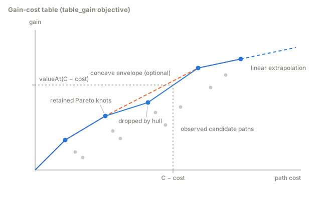
table_gain replaces the extrapolation of expected_gain with the gain-cost table (GainCostTable): every candidate path scored under table_gain adds a (cost, gain) knot, a knot is dropped when another at no more cost has at least its gain, and with concave_envelope (default true) the rest are reduced to their upper concave hull. The table interpolates linearly from (0,0), extrapolates along its last segment, and is cleared each episode. Candidates are scored against the table built so far, so table_gain depends on the search order.

Ties and the Fallback Step

Exact ties go to a frontier end under expected_gain and table_gain, then to the higher ratio, the higher gain and the lower cost. The beams of nbs and dbs are ranked by ratio, gain and lower cost whatever the objective; the objective only picks the answer. When the search keeps no path, for example because every path exceeds the remaining budget, the path planner returns a one-edge step to a random neighbor so the robot keeps moving.

Beam Search Complexity

As shipped (check_previous_path: false, no gain suppression), DBS and NBS run Algs. 1 and 2 of the paper unchanged: the same expansions in the same order, the same preference operator and the same selection criteria. Only the bookkeeping of a path differs. In the paper, extending a path copies it and scans it for a revisit, O(D) each time. Here a path is its cost, gain and last step, and paths share their common prefix as a chain of steps, so an extension adds one step in O(1). When a path is expanded, its steps are walked once, O(D), marking on the graph the nodes it visited; each of its extensions then checks a mark in O(1). The marks live on the graph, so one search runs on a graph at a time.

In theory. In the notation of the paper’s Table 1 (graph G = (V, E), beam width B, depth D):

Alg.	Time, paper	Time, this release	Space, paper	Space, this release
DBS	O(|V| D B (D + log B))	O(D B (D + |V| log B))	O(D B)	O(|V| D B)
NBS	O(|E| D B (D + log B))	O(D B (|V| D + |E| log B))	O(|V| D B)	O(|E| D B)

Time: the O(D) term moves from every extension to every expanded path, so per path it shrinks by the branching factor, |V| for DBS and |E| / |V| for NBS. Space: a step is kept until the search returns, because other paths may share it, so the bound is one step per extension that entered a beam or became the best path, above the paper’s live-beam bound. With is_gain_correlated, where a node holds A gain anchors, the walk costs O(D A) and a gain check O(A).

In practice. About one extension in six keeps its step, and the shared steps take less memory than the copies did. On a synthetic graph of 65 positions × 32 orientations with four shared anchors each (NBS, B = 1, D = 200), one search takes 0.33 s and 13.6 MB instead of 4.0 s and 40.9 MB. The gain grows with path length.

Graph benchmark. The DBS, NBS and SPT result files of all eight datasets match the paper’s file by file: the same paths and the same gains. Their cost budgets stop paths at about 15 edges, long before D, so the planning time is within 3 % of the implementation behind the paper on six of the eight datasets.